AIPS Calibration Workflow
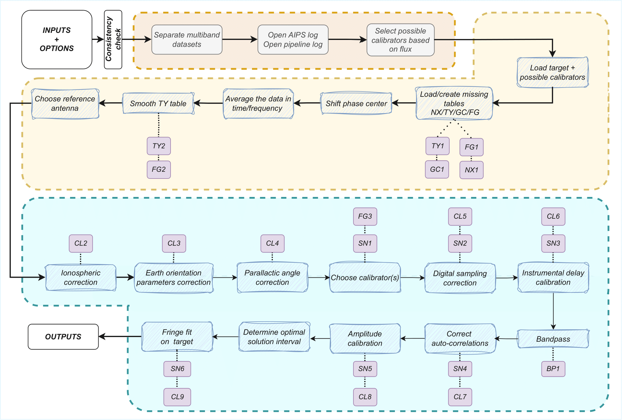
In this section, we provide a detailed description of the AIPS tasks used throughout the pipeline, along with their most relevant parameters. For the scientific motivation behind this workflow, please refer to Alvarez-Ortega et al. (2025).
Data loading
After splitting in frequencies and selecting multiple potential calibrators, data are loaded into AIPS using FITLD:
task 'FITLD'

outname       # Project name
outdisk
outclass      # The loaded frequency, i.e. 22G for K band data
outseq    1

sources       # Science targets + potential calibrators
bif           # Depending on frequency loaded
eif           # Depending on frequency loaded
clint     0.1 # CL entry interval in minutes
selfreq       # Depending on frequency loaded
fqtol         # 0.5% of selfreq
If more than 1 file is loaded, redundant calibration tables are merged with TAMRG
# GC tables
task 'TAMRG'

inext     'GC'
aparm     1 1 2 1 3 1
bparm     1 2 3

invers    1
outvers   1
# TY tables task 'TAMRG' inext 'TY' aparm 1 1 4 1 5 1 6 1 bparm 1 3 4 5 6 cparm 0.1/(24*60*60) # Tolerance for timestamps, 0.1s invers 1 outvers 1# PC tables task 'TAMRG' inext 'PC' aparm 1 1 4 1 5 1 6 1 bparm 1 3 4 5 6 cparm 0.1/(24*60*60) # Tolerance for timestamps, 0.1s invers 1 outvers 1
Pre-calibration checks
If the loaded data not in time-baseline (TB) order, they are sorted with UVSRT
task 'UVSRT'

sort  'TB'
If there is not an index table (NX) or an intial calibration table (CL1), they are created with INDXR
task 'INDXR'

cparm(3)  0.1 # CL entry interval in minutes
cparm(4)  4   # Recalculate CL group delays if IM table is available
Table loading
When system temperatures (TY1), gain curves (GC1), or initial flag tables (FG1) are not available in the data, they are retrieved online and loaded using ANTAB
task 'ANTAB'

tyver 1
gcver 1
calin     # Tsys or GC file
or UVFLG in case of the initial flag table
task 'UVFLG'

intext    # Flag file
When the dataset has been observed with the VLBA and the calibration tables have been generated with the TSM software, the pipeline uses the VLOG task to extract the information
task 'VLOG'

calin     # cal.vlba file
outfile   # Path for the extracted tables in ANTAB format
If there are non-ASCII characters in the antenna table (AN), these are replace with the correct values. This is done to avoid issues with ParselTongue, and the TABED task can be used for this purpose
# For antenna names

task 'TABED'

inext     'AN'
invers    1
outvers   1
optype    'REPL'

aparm(1)      # Column to modify, 1 for ant names, 9 for pol names
aparm(2)  0   # First character to modify
aparm(3)  0   # Last character to modify
aparm(4)  3   # String type

bcount        # Iterate over all rows one by one
ecount        # Same row as bcount

keystrng      # Correct names, extracted from the fits file
# For polarization names task 'TABED' inext 'AN' invers 1 outvers 1 optype 'REPL' aparm(1) 9 # Column to modify, antenna names are 1 aparm(2) 0 # First character to modify aparm(3) 0 # Last character to modify aparm(4) 3 # String type bcount # Iterate over all rows one by one ecount # Same row as bcount keystrng # Correct antenna names, extracted from the fits file
Phase center shift
If specified by the user, VIPCALs can shift the correlation phase center of a source. It can be done through the UVFIX task, going from the old coordinates RA, DEC, to the new ones RA’, DEC’.
task 'UVFIX'

srcname   # Target to shift
shift     # shift_1, shift_2
where shift_1 = cos(DEC) * (RA’ - RA), and shift_2 = (DEC’ - DEC).
Time/frequency average
To improve the signal-to-noise ratio while still preserving coherence, VIPCALs can apply both a time and frequency average. By default, if the time sampling is shorter than 1s, data are averaged in 2s bins with UVAVG
# GC tables
task 'UVAVG'

doacor    1   # Keep autocorrelations
yinc      2   # Final sampling time, can be changed
zinc          # Original sampling time
opcode    'TIME'
In frequency, the pipeline will run AVSPC by default if the channel width is narrower than 0.5MHz.
# GC tables
task 'UVAVG'

doacor    1   # Keep autocorrelations
channel       # Ratio old_channels/new_channels
avoption  'SUBS'
After this steps, the scan list is printed with LISTR into a text file in the output folder
task 'LISTR'

optype    'SCAN'
flagver   1
xinc      1   # Display all lines
docrt     -2  # Print to external file
TY table smoothing
System temperatures are filtered and smoothed using TYSMO. Default criteria are to flag temperatures below 0K, over 1500K, and that deviate more than 250K from the mean of a given source
task 'TYSMO'

invers    1
outvers   2

inext     'TY'
dobetween 0       # Smooth each source individually

aparm(1)  0       # Minimim temperature
aparm(6)  1500    # Maximum temperature

cparm(1)  15      # Time interval in which the mean is computed
cparm(6)  250     # Maximum deviation allowed with respect to the mean
Antennas with no TY or GC tables at this stage, or where all Tsys values have been flagged, are flagged in FG2 using UVFLG. First, FG1 is copied into FG2 using TACOP.
# Copy the table

task 'TACOP'

inext     'FG'
invers    1
outvers   2
# Flag the antennas task 'UVFLG' antennas # Antennas with no TY or GC outfgver 2 reason 'NO TSYS/GC'
TSys tables, both original and smoothed, are plotted with SNPLT
task 'SNPLT'

inext     'TY'
optype    'TSYS'
invers        # 1 or 2
nplots    8
dotv      -1
and then printed to a PostScript file with LWPLA
task 'LWPLA'

dparm 0 0 0 0 0 4 31 7 0  # Plotting parameters
Choice of reference antenna
A fringe fit with FRING is run on a selected number of scans, rotating around all possible reference antennas. This allows the pipeline to assign a fringe S/N to each antenna.
task 'FRING'

refant        # Rotates around antennas
docalib   1   # Use calibrated data
gainuse   1
solint        # Scan length
timeran       # Scan time

aparm(1) 2    # Min. number of antennas for a solution
aparm(5) 0    # Solve IFs separately
aparm(6) 2    # Amount of information printed
aparm(7) 1    # No S/N cutoff

dparm(1) 1    # Number of baseline combinations
dparm(2) 1000 # Delay window in ns
dparm(3) 200  # Rate window in mHz
dparm(5) 1    # Stop at the FFT stage
This is run on a selected number of scans per each antenna, and each antenna gets all the solution tables merged into one. It is done with CLCAL.
task 'CLCAL'

opcode 'MERG'
snver     # First SN table of the antenna
invers    # Last SN table of the antenna
refant    # Each antenna
Only the merged table is kept, the rest are deleted.
Ionospheric delay correction
Data observed after June 1998 are corrected for ionospheric delays. This is done with TECOR. Files are obtained from NASA
task 'TECOR'

infile        # Depends on the date
nfiles        # Number of days observed
aparm(1)  1   # Correct for dispersive delays
gainver   1   # From CL1
gainuse   2   # To CL2
The IONEX file used is infile is codgDDD0.YYi for observations older than GPS Week 2238 (26/11/2022), and COD0OPSFINYYYYDDD0000_01D_01H_GIM.INX for newer observations. DDD, YY, and YYYY refer to the day, 2-digit year, and 4-digit year of the observation.
Files older than June 1998 simply get their CL1 copied into CL2 with TACOP.
Geometric corrections
Earth orientation parameters and parallactic angle are corrected for with CLCOR.
# EOPS
task 'CLCOR'

opcode    'EOPS'
clcorprm  3 7     # Consider data from +- 3 days
infile            # usno_finals_bis.erp provided by the USNO

gainver 2         # From CL2
gainuse 3         # To CL3
# Parallactic angle task 'CLCOR' opcode 'PANG' clcorprm 1 0 # Add corrections gainver 3 # From CL3 gainuse 4 # To CL4
Choice of calibrator scans
The pipeline uses FRING to rank each scan based on its fringe S/N
task 'FRING'

refant        # Reference antenna
docalib   1   # Use calibrated data
gainuse   4   # Use CL4
solint        # Scan length

aparm(1) 2    # Min. number of antennas for a solution
aparm(5) 0    # Solve IFs separately
aparm(6) 2    # Amount of information printed
aparm(7) 5    # S/N threshold
aparm(9) 1    # Use other antennas as backup reference antennas
search        # Prioritized list of antennas to use

dparm(1) 1    # Number of baseline combinations
dparm(2) 1000 # Delay window in ns
dparm(3) 200  # Rate window in mHz
dparm(5) 1    # Stop at the FFT stage

snver 1       # Produce SN1
If, for a certain antenna, there are no scans with S/N greater than 5, then that antenna is flagged in FG3 using UVFLG
task 'UVFLG'

antennas      # Antennas with no reliable calibrators
outfgver  3
reason    'NO CALIB'
Digital sampling correction
Autocorrelations are normalized using the ACCOR, with corrections being applied with CLCAL
task 'ACCOR'

solint    10      # Solution interval of 10 minutes, not respecting scan boundaries
task 'CLCAL' opcode 'CALP' interpol 'SELF' snver 2 gainver 4 # From CL4 gainuse 5 # To CL5
Instrumental delay correction
FRING is run for each of the calibrator scans selected previously.
task 'FRING'

refant        # Reference antenna
docalib   1   # Use calibrated data
gainuse   5   # Use CL5
solint        # Scan length

calsour       # Calibrator source
timerang      # Scan interval
antennas      # refant + antennas to be calibrated

aparm(1) 2    # Min. number of antennas for a solution
aparm(5) 0    # Solve IFs separately
aparm(6) 2    # Amount of information printed
aparm(7) 5    # S/N threshold
aparm(9) 1    # Use other antennas as backup reference antennas
search        # Prioritized list of antennas to use

dparm(1) 1    # Number of baseline combinations
dparm(2) 1000 # Delay window in ns
dparm(3) 200  # Rate window in mHz
dparm(8) 1    # Zero the rated after fitting

snver 3       # Produce SN3
If there is more than one calibrator scan, merge the solutions with CLCAL
task 'CLCAL'

opcode    'MERG'
snver     3
invers    3+n
refant        # Reference antenna
And apply the solutions with CLCAL
task 'CLCAL'

opcode    'CALP'
interpol  '2PT'
snver         # Merged SN table
gainver   5   # From CL5
gainuse   6   # To CL6
If there were multiple calibrator scans, the individual tables are removed and the merged table is copied to SN3.
Complex bandpass
Bandpass is corrected with BPASS
task 'BPASS'

solint        -3      # Solution interval respecting scan boundaries
refant            # Reference antenna
calsour           # Calibrator sources

docalib       1   # Use calibrated data
gainuse       6   # Use CL6
outvers       1   # Produce BP1

solint        -1  # Scan length
weightit      1   # Weight data by 1/sigma
bpassparm(5)  0   # Divide by channel zero (central 75% of the IF)
bpassparm(9)  1   # Interpolate over flagged channels

# If only one calibrator scan is used:
timerang          # Time interval of the scan
bpassparm(10) 6   # Shift the average phase to 0
After the bandpass corrections, normalize again the autocorrelations with ACSCL. Solutions are applied with CLCAL.
task 'ACSCL'

solint    10      # Solution interval of 10 minutes, not respecting scan boundaries
docalib   1   # Use calibrated data
gainuse   6
doband    1   # Apply bandpass correction
task 'CLCAL' opcode 'CALP' interpol 'SELF' snver 4 gainver 6 # From CL6 gainuse 7 # To CL7
Amplitude calibration
Final amplitude calibration is computed with APCAL and applied with CLCAL
task 'APCAL'

solint    -3  # Solution interval respecting scan boundaries
task 'CLCAL' opcode 'CALP' interpol 'SELF' snver 5 gainver 7 # From CL7 gainuse 8 # To CL8
Target fringe fit
Before running the final fringe fit, the solution interval is optimized by running a fringe fit in a reduced set of target scans.
task 'FRING'

refant            # Reference antenna
calsour           # Science target or phase-reference calibrator

solint            # Rotates between 5, 4, 3, 2, and 1 solutions per scan

docalib   1     # Use calibrated data
gainuse   8     # Use CL8
doband    1     # Apply the bandpass correction

aparm(1) 2    # Min. number of antennas for a solution
aparm(5) 0    # Solve IFs separately
aparm(6) 2    # Amount of information printed
aparm(7) 1    # No S/N threshold
aparm(9) 1    # Use other antennas as backup reference antennas
search        # Prioritized list of antennas to use

dparm(1) 1    # Number of baseline combinations
dparm(2) 1000 # Delay window in ns
dparm(3) 200  # Rate window in mHz
dparm(5) 1    # Stop at the FFT stage
Finally, fringe fit on target (or phase reference source) to correct for residual delay and rates
task 'FRING'

refant            # Reference antenna
calsour           # Science target or phase-reference calibrator

solint            # Optimal solution interval
docalib   1     # Use calibrated data
gainuse   8     # Use CL8
doband    1     # Apply the bandpass correction


aparm(1) 2    # Min. number of antennas for a solution

# On a first round
aparm(5) 0    # Solve IFs separately
# On a second round
aparm(5) 1    # Solve IFs together

aparm(6) 2    # Amount of information printed
aparm(7)      # S/N cutodd, default is 5
aparm(9) 1    # Use other antennas as backup reference antennas
search        # Prioritized list of antennas to use

dparm(1) 1    # Number of baseline combinations
dparm(2) 1000 # Delay window in ns
dparm(3) 200  # Rate window in mHz
Solutions are applied with CLCAL
# If the fringe fit is on the science target

task 'CLCAL'

opcode    'CALP'
interpol  'SELF'
cutoff        # 1.1*scan_length, interpolate solutions only within the scan
gainver   8   # From CL8
gainuse   9   # To CL9
# If the fringe fit is on the phase-reference calibrator task 'CLCAL' sources # Science target opcode 'CALP' interpol '2PT' gainver 8 # From CL8 gainuse 9 # To CL9
Data export
Calibration, flags, and bandpass corrections are applied with SPLIT. Final calibrated data are exported to a uvfits with FITTP
task 'SPLIT'

sources       # Science_target
docalib   1   # Use calibrated data
gainuse   9   # Use CL9
doband    1   # Do bandpass
fgver     3   # Use the last FG table

# If channel_out == 'SINGLE'
aparm(1)  2
# If channel_out == 'MULTI'
aparm(1)  1

bchan         # Initial channel to calibrate, by default 1
echan         # Final channel to calibrate, by default the last
task 'FITTP' dataout '/output_folder/sourcename_project_band_date/sourcename_project_band_date.uvfits
Plots
PostScript format plots are produced from AIPS using different tasks.
For amplitude and phase as a function of frequency, both uncalibrated and calibrated, POSSM is used.
task 'POSSM'

sources           # Science target
stokes    'RRLL'
solint    -1      # Scan length

docalib   1       # Use calibrated data
gainuse           # 1 for the uncalibrated, 9 for the calibrated
flagver           # 1 for the uncalibrated, 3 for the calibrated
doband            # 0 for the uncalibrated, 1 for the calibrated

bchan             # Initial channel to calibrate, by default 1
echan             # Final channel to calibrate, by default the last

# Plotting options
aparm 1 1 0 0 -180 180 0 0 1 0
nplots 9
dotv -1
For calibrated amplitudes and phases as a function of time, the pipeline uses VPLOT
task 'VPLOT'

sources           # Science target

avgchan   1       # Average channels
avgif     1       # Average channels
solint    0.09    # One point every 5 seconds

docalib   1       # Use calibrated data
gainuse   9       # Use CL9
flagver   3       # Use FG3
doband    1       # Correct for bandpass

bchan             # Initial channel to calibrate, by default 1
echan             # Final channel to calibrate, by default the last

# Plotting options
bparm 12 -1 0
nplots 2
dotv -1
For the uv coverage, the pipeline uses UVPLT
task 'UVPLT'

sources           # Science target
stokes    'RRLL'
solint    0.09    # One point every 10 seconds

docalib   1       # Use calibrated data
gainuse   9       # Use CL9
flagver   3       # Use FG3
doband    1       # Correct for bandpass

bchan             # Initial channel to calibrate, by default 1
echan             # Final channel to calibrate, by default the last

# Plotting options
bparm 6 7 2 0
do3color -1
dotv -1
Finally, all these plots are printed into PostScript files using LWPLA
task 'LWPLA'

# Plotting options
dparm     0 0 0 0 0 4 31 7 0